Expected Resolution of a GPR Survey
The structures that we will be able to see with a GPR survey depend on the system that we use as well as on subsurface properties. From the seven step framework you learned how important it is to assess whether a survey will be successfull before collecting data in the field. In this section you will learn how to determine what GPR system to use in which situation and what size of structure you can expect to resolve.
Source Signal
As we have already discussed, the source antenna sends a pulse of radiowaves into the ground. Radiowaves carry oscillating electric and magnetic fields. As it turns out, the pulse is not made up entirely of radiowaves of a single frequency. Instead, a set of sinusoidal EM waves of similar frequencies are used create what is called a wavelet. As a result, the wavelet contains information over a range of frequencies (generally between \(10^6\) and \(10^9\) Hz).
Before we move forward let us define a few terms:
Wavelet: A wave-like oscillation of short duration.
Bandwidth: The range of frequencies present in the source wavelet.
Pulse Width: The time duration of the wavelet.
Spatial Length (wavelength): The physical length of the wavelet signal while it propagates through a medium.
Central Frequency: The central frequency corresponding to the bandwidth. In general, the central frequency defines the propagation of the GPR signal.
GPR Signals and Bandwidth
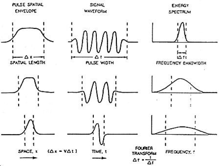
The figure below can be used to examine the relationships between the 5 aforementioned terms. As we can see, the bandwidth and central frequency for the GPR signal depend on the pulse width of the wavelet. Here are a few important relationships to keep in mind:
1) For a pulse width \(\Delta t\), the central frequency \(f_c\) is given by:
As a result, longer wavelets generally contain lower-frequency information. Frequencies corresponding to GPR signal are around 100 MHz to 1 GHz. This results in pulse widths around 1 ns to 10 ns.
2) The bandwidth increases as the pulse width decreases. In order to create a wavelet with a longer pulse width, only frequencies near the central frequency are needed. However, a large range of frequencies (or bandwidth) is needed to create wavelets that have short pulse widths.
3) The spatial length (wavelength) increases as the pulse width increases. As we can see from the figure below, the “wave envelope” is longer for wavelets that have a long pulse width.
GPR Signals and Spatial Length
The spatial length of the GPR wavelet signal is different as it moves through different materials. For a wavelet with central frequency \(f_c\) moving at velocity \(V\), the wavelength \(\lambda\) is given by:
where \(c = 3.00 \times 10^8\) m/s is the speed of light and \(\varepsilon_r\) is the relative permittivity. This expressions shows that if the signal is moving through a material with a higher dielectric permittivity, it will move slower and it will have a larger spatial width. It also shows that GPR signals with higher central frequencies have shorter spatial widths.
Recall that the central frequency is the reciprocal of the pulse width (\(f_c = 1/\Delta t\)). Thus:
Therefore, shorter pulse widths result in shorter spatial lengths. This was stated in the previous subsection.
Examine the animation below. Observe the wave as it propagates through both the ground and the Earth. In which medium is the wavefront thicker/thinner? In which medium is the GPR signal moving slower/faster? Does this make sense from the equations above?
Survey Resolution and Probing Distance
The pulse width, and thus the frequency content contained within the GPR signal, is a very important aspect of planning a GPR survey. The concepts of resolution and probing distance are discussed here.
Vertical Resolution for Layers
Resolution defines the smallest features which can be distinguished in a GPR survey. The vertical resolution for GPR surveys depends on the pulse width of the signal.
In order for a layer to be detected using a GPR survey, it must be sufficiently thick compared to the wavelength of the incoming wavelet. As a general rule, the layer must be at least 1/4 the wavelength of the incoming wavelet to be detectable. Thus:
where \(L\) is the layer thickness, \(c/\!\sqrt{\varepsilon_r}\) is the propagation velocity for radiowaves, \(\Delta t\) is the pulse width and \(f_c\) is the central frequency. As we can see from this expression, higher frequencies/shorter pulse widths are required to observe smaller features. This means higher frequencies/shorter pulse widths are used for higher resolution surveys.
Horizontal Resolution for Objects
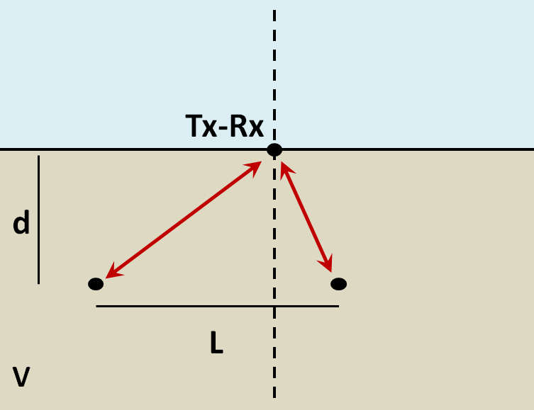
When the resolution of the survey is sufficient, returning signals from separate buried objects are distinguishable. However, if buried objects are too close to one another, their respective returning GPR signals can be hard to differentiate. In general, we can distinguish the signals from two nearby objects so long as:
where \(V\) is the propagation velocity, \(f_c\) is the central frequency for the wavelet, \(d\) is the depth to the objects and \(L\) is the separation distance from both objects. We can see from this equation, that by reducing the pulse length, we can see objects that are closer together. Additionally, it is harder to distinguish objects which are further away from the transmitters and receivers.
Attenuation
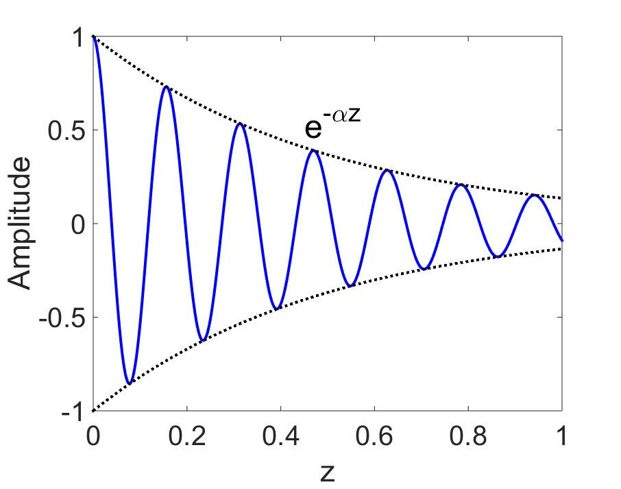
Fig. 15 Attenuation of electromagnetic waves.
Attenuation defines the continuous loss of amplitude a wave experiences as it propagates through a particular medium. The rate at which the amplitude decreases is referred as the attenuation constant (\(\alpha\)). For an electromagnetic wave that has traveled a distance \(z\), the attenuation constant is given by:
where \(\mathbf{A_0}\) is the initial amplitude of the wave and \(\mathbf{A}\) is the amplitude of the wave after it has travel distance \(z\). We can see that as \(z \rightarrow \infty\), the amplitude of the wave goes to zero. Additionally, for larger values of \(\alpha\), the wave attenuates more quickly.
The attenuation constant depends on the physical properties of the media. In general, the attenuation constant can be expressed as:
In this formula, \(f_c\) is the center frequency of the GPR signal. It is important to note that for low electrical conductivities \(\sigma\), i.e., electrically resistive materials (the second case in the equation above), the attenuation does not depend on the frequency. This means that we can use high frequency systems and increase the resolution without reducing the depth of investigation (as long as the condition \(\sigma \ll 2\pi f_c \varepsilon\) is met). This is why GPR works so well for sand or ice, where we can resolve fine details at great depth. On the other hand, for electrically conductive materials (high values for \(\sigma\)), the signal does not get very deep. This is the reason why GPR does not work well for clay, unless we use a system with a low enough \(f_c\) to reduce the value of \(\alpha\). But then, we won’t resolve much detail.
Skin Depth
Skin depth (\(\delta\)) defines the propagation distance at which the amplitude of an electromagnetic wave is reduced by a factor of \(1/e\); i.e. reduced to 37% of its original amplitude. By definition, the skin depth is just the reciprocal of the attenuation constant:
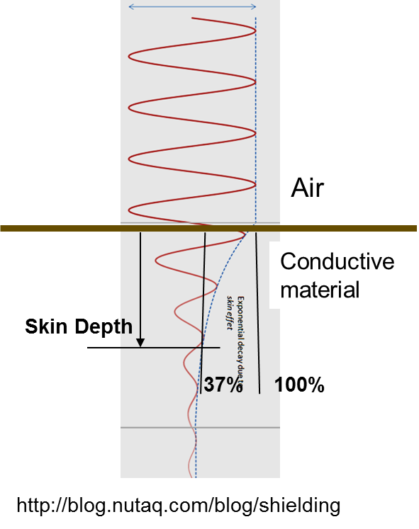
Fig. 16 Figure comparing the attenuation of radiowaves in air versus in a conductive medium.
If we use the approximations found above and assume the Earth is non-magnetic (\(\mu_r = 1\)), the skin depth is given by:
Where \(f\) is the frequency of the wave in Hz. We can see from the two previous expressions that:
Generally, the skin depth is smaller if the frequency of the electromagnetic waves is higher.
For the wave regime approximation (\(\sigma \ll \omega \varepsilon\)), skin depth reaches a limit which doesn’t depend on frequency.
The skin depth is larger in materials with lower conductivities.
The skin depth is larger is materials with higher dielectric permittivities.
An example of the attenuation of electromagnetic waves in air versus inside a conductive is shown on the right. We can see that in the air, the wave experienced little to no loss in amplitude as it propagates. In the conductive material however, the amplitude of the wave decreases noticeably as it propagates.
Probing Distance
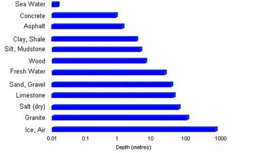
Fig. 17 Proving distances for GPR signals for various materials.
Probing distance characterizes the maximum depth in which GPR signals can be used to obtain information about subsurface structures. For materials which have larger skin depths, radiowaves can penetrate deeper into the ground and still provide a sufficiently strong returning signal.
As a general rule, the probing distance (\(D\)) is approximated 3 skin depths. If we assume the Earth is non-magnetic (\(\mu_r = 1\)):
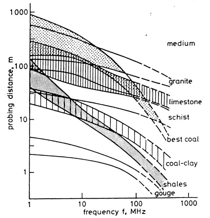
Fig. 18 Probing distance for various materials from 1 MHz through 1 GHz.
On the right we see figures which show probing distances for various materials. Using these figures, we can see that:
In general, as the frequency increases, the skin depth decreases and the probing distance decreases.
Frequencies used for GPR are \(\sim\) 1 GHz. Therefore, the probing distances for GPR signals are generally quite shallow.
It is very difficult for GPR signals to penetrate concrete and asphalt, as the probing distance is only about 1 m for GPR.
Water saturated sedimentary rocks, such as clays and sandstones, have much lower probing distances than dry sedimentary rocks.
Rocks saturated with sea water have much smaller probing distances than rocks saturated with fresh water.
The probing distances for hard rocks (granites, limestones, schists…) is quite large.
Probing Distance versus Resolution
On the right we see several radargrams corresponding to data collected over two buried tunnels (hyperbolic features). Each radargram was collected using a different frequency.
By using a 200 MHz central frequency, we are hoping to obtain a high resolution radargram. However, the attenuation of radiowaves is more severe at higher frequencies. As a result, the GPR signal does not penetrate deep enough to image either of the tunnels. At 100 MHz, both tunnels become partially visible in the radargram (hyperbolic signatures). This is made possible because because the probing distance is larger. In the 50MHz radargram, both tunnels are easily recognizable. This is made possible because the probing distance is now large enough. Notice however, that the hyperbolic features in the radargram are slightly less distinct.
We can see from this example that there is a compromise between resolution and probing distance. It is important to choose a frequency which is high enough to image sufficient small features. However, the probing distance of the background medium must be large enough to obtain a return signal.
Reflection and Transmission of Radiowaves
When a radiowave reaches an interface, some of it is reflected and some of it is transmitted across the interface. This results in both a reflected and a transmitted wave.
The amplitude of the reflected wave proportional to that of the incident wave is defined by the reflection coefficient (\(R\)). For radiowaves, the reflection coefficient can be expressed as a function of the relative permittivities on each side of the interface. Assuming the radiowave arrives at an angle perpendicular to the interface, the reflection coefficient is given by:
where \(\varepsilon_1\) is the relative permittivity of the medium carrying the incident and reflected waves. The transmission coefficient is given by:
The reflection coefficient can be either positive or negative and has values between \(-1 < R < 1\). The magnitude of \(R\) determines how much of the incident wave is reflected. It should be noted that:
If \(\varepsilon_1\) and \(\varepsilon_2\) are similar, most of the incident wave is transmitted through the interface.
If one of the relative permittivities across the interface is much smaller than the other, most of the incident wave is reflected. This can be a problem if you at attempting to gain information about structures below this interface.
The sign of the reflection coefficient determines whether the reflected wave experiences a reverse in polarity. As a result, we can use the polarity of reflected radiowaves to determine whether \(\varepsilon_1\) is greater than or less than \(\varepsilon_2\). This can be summarized as follows:
If the returning signal (reflected wave) shows a reverse in polarity, \(R<0\) and thus \(\varepsilon_1 < \varepsilon_2\)
If the returning signal (reflected wave) does not show a reverse in polarity, \(R>0\) and thus \(\varepsilon_1 > \varepsilon_2\)
Examine the GIF in fig_gpr_layeredearth_gif.
Look at the reflected wave as it returns to the surface.
When it reaches the surface, is most of the wave reflected or transmitted?
From this, are the relative permittivities of the air and the ground very different or similar?
GPR and Sources of Noise
Noise is used to describe any measured signal which does not correspond to signals from desired targets. When the sources of noise are sufficiently large, it can be difficult to identify and classify signals in radargrams. That is why it is necessary to take steps which minimize the impact of external noise sources on the data. Below are some sources of noise relevant to GPR and their impact.
Radiowaves from Other Sources
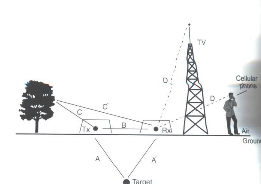
Fig. 23 Some external sources of noise related to GPR system, which can be reduced through shielding.
Much of 21st century communication is made possible with radiowaves. Cellular phones, radio towers and other transmitting systems all use radiowave frequencies to transmit information through the air. These signals can be measured by the receiver and have the potential to mask responses from desired targets. To limit the effects of external sources, the transmitter and receiver are frequently protected by a shield (as depicted in the image).
Returning Signals from Above-Ground Objects
GPR is used to gain information about structures below the Earth. However, since radiowaves propagate through the air, it is possible to measure returning signals from nearby objects as well. This is common in urban and wooded environments where GPR signals can reflect off of buildings and trees.
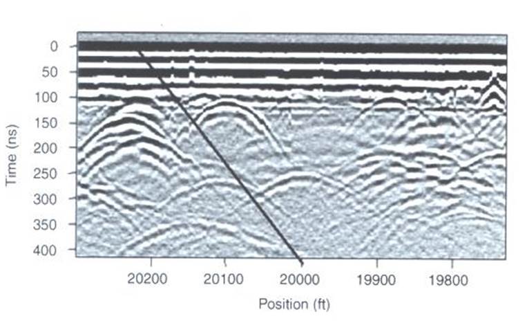
Fig. 24 Zero-offset radargram example containing returning signals from nearby trees.
On the right, we see an example of a radargram for a zero-offset configuration. The survey was performed in a wooded area without using a shield. Because the trees acts as point reflectors, they produce hyperbolic signatures in the radargram. Using the slope on either end of the hyperbola, we find that the propagation velocity associated with this reflection is \(2/c\); this is demonstrated with a line. This verifies that the signature must correspond to an object which is above the ground. And we can infer that signatures after 100 ns correspond to nearby trees.
Below, we show the two-way travel path for reflected signals off a tree and a building. A diagram showing the different radargram signatures for both the tree and the building is also provided. Unlike the tree, the face of the building is not a point reflector. However, the ends of the signature corresponding to the building also have slopes which are \(2/c\). Thus, we can infer the propagation velocity.
To avoid measuring signals such as these, shields may also be used on the transmitter and receiver. However, if signals from above ground objects are present in the radargram, they can be be identified for zero-offset configurations by their slope.
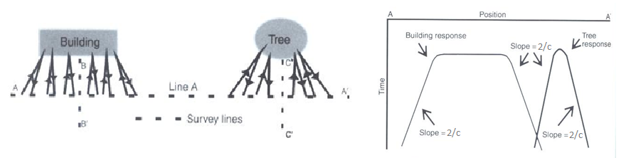
Fig. 25 Zero-offset radargram example for returning signals from a tree and building wall.
Ringing
Ringing occurs when radiowave signals reverberate in regular fashion. This is created when GPR signals repeatedly bounce within or between nearby objects. In response to ringing, the returning signal from a particular interface(s) is not ‘sharp’ in the radargram. Instead, it becomes present over all times.
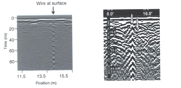
Fig. 26 (Left) Radargram showing ringing from a small metal wire near the surface. (Right) Ringing from two nearby objects.
Noise from Scattering
Scattering is used to describe deviations in the paths of electromagnetic waves due to localized non-uniformities; which are less than 1/4 the wavelength of the radiowave signal. Scattering is problematic for GPR because it reduces the amplitudes of useful signals while increasing extraneous noise. If the Earth is made up of homogeneous units, scattering is negligible and returning GPR signals are easily visible. If the Earth is very inhomogeneous, the effects of scattering may produce significant extraneous noise.
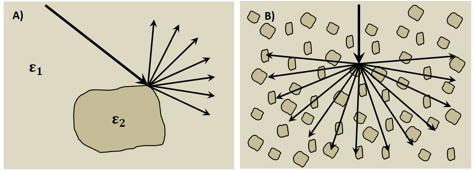
Fig. 27 Examples of scattering. A) Scattering from irregular surface texture. B) Scattering in rocky soils.
Below, we show a representation of data from a single Tx-Rx shot. On the left, scattering is negligible and the returning wavelet is easily visible. On the right, the returning wavelet is hard to see due to incoherent noise cause by scattering. In addition, we see that the amplitude of the returning wavelet signal is less, as scattering resulted in a loss in amplitude.
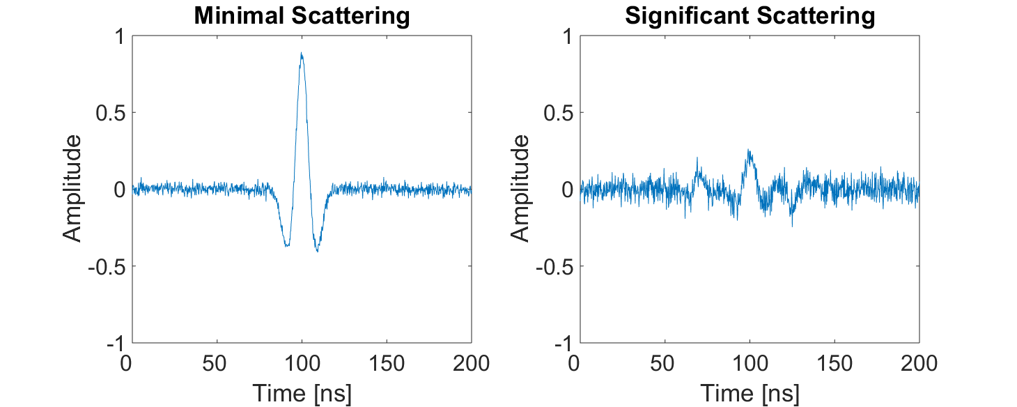
Fig. 28 Return signals with different levels of scattering noise (Left) Minimal noise. (Right) Significant scattering noise.