Surveys and Data

Here, we discuss the various survey geometries used in GPR and some of their applications. Information about the GPR source signal and its impact on planning surveys is presented. We also discuss sources of noise which may contaminate GPR data.

On this page, you will learn about:

• Common offset, common midpoint and transillumination surveys.

• Where these surveys are most effective.

• What is the source signal used in GPR.

• The properties of the source signal and how it impacts the effectiveness of GPR surveys.

• The resolution of GPR surveys.

• The probing distance of GPR surveys.

• Sources of noise and their impact on GPR surveys.

Wave Fronts and Ray Paths

A wavefront indicates the set of locations at which the phase of the wave has the same value. For example, visualize the peaks (or troughs) of water ripples after a rock has been thrown into a pond. Rays are imaginary lines perpendicular to the wavefront that indicate the path along which the wavefront is traveling. Rays are not physical entities. They exist only to illustrate where the energy travels. It is important to remark here that the arrival of energy at a sensor is not a point event. The energy is spread in space and time. Note how the peaks and troughs of the waves on the pond have widths, which remains constant as they propagate. Similarly, the radar wave will arrive at a sensor as a pulse of energy with some shape and width, not as a spike occurring a single instance in time. This pulse of energy is called a wavelet.

To summarize:

• Wave-front: The physical location of the radiowave signal as it propagates through the Earth.

• Ray path: A particular path which a portion of the wave-front can take in order to reach a particular location.

Thus the wave-front represents the actual pulse of radiowaves, and the ray path is used to represent paths which signals can take to reach a receiver location. To follow a ray path, choose a small sliver of the wavefront and follow it as it reflects and propagates. If at any time this portion of the wavefron reaches a sensor, it is a ray path which is measured.

Common Offset Survey

Fig. 12 Common offset survey configuration.

Common offset surveys are the most frequently used configuration for GPR surveys. In common offset survey, the distance between the transmitter and a single receiver is fixed. Data are collected each time the transmitter-receiver pair are moved to a new position. In some cases, the transmitter and receiver are placed at a zero-offset; otherwise known as a coincident source and receiver.

Common-offset surveys are effective for locating the depths of approximately horizontal interfaces. In addition, zero-offset surveys are very affective a locating pipes, tunnels and compact buried objects; as they generate hyperbolic signatures in radargram data. Examples of this can be seen below.

Buried Compact Objects

Below we see the geometry for a zero-offset survey and the corresponding radargram. We will show how the geometry of the problem and the radargram can be used to resolve the locations of pipes and blocky objects.

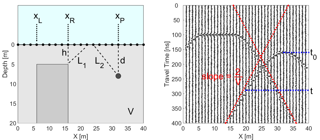
Fig. 13 (Left) Problem geometry showing a buried pipe and a block. (Right) Corresponding radargram for the problem geometry.

In GPR, a thin pipe will act as a point reflector. According to the geometry of the problem, the total travel time of the GPR signal as it reflects off the pipe is given by:

\[t_p = \frac{2 L_2}{V} = \frac{2 \sqrt{ (x - x_p)^2 + d^2}}{V}\]

where \(V\) is the propagation velocity (light gray region) and \(d\) is the depth to the pipe. The propagation velocity (or “radar wave velocity”) \(V\) depends on the subsurface material. The next section Propagation Velocities contains a lookup table for the velocity for various subsurface materials.

As we can see in the radargram, the arrival times for a compact object form a hyperbola. When we are directly above the pipe (\(x = x_p\)), the total travel time is smallest and equal to:

\[t_p (x_p) = \frac{2 d}{V}\]

For the block, things are a little more complicated. Above the face of the block (\(x_L\) = 6 m to \(x_R\) = 16 m), the signal measured by the receiver reflects directly. However, the return signal at locations outside the margins of the block occur on the points. As a result, the total travel time for reflected signals off the block are given by:

\[\begin{split}t_b = \begin{cases} \dfrac{2 \sqrt{(x-x_L)^2 + h^2}}{V} \;\;\; &\textrm{for} \;\;\; x < x_L \\ \dfrac{2h}{V} \;\;\; &\textrm{for} \;\;\; x_L \leq x \leq x_R \\ \dfrac{2 \sqrt{(x-x_R)^2 + h^2}}{V} \;\;\; &\textrm{for} \;\;\; x > x_R \end{cases}\end{split}\]

where \(h\) is the depth to the top of the block. As we can see from the previous equation, we expect to see a flat feature the block’s radargram signature. Then on either size of the block, the radargram signature resembles one-half of a hyperbola.

Resolving Buried Objects: Method 1

In order to locate buried objects, we first need to use the radargram to obtain a velocity for the medium. Let us begin by considering the pipe. Notice that at large offset distances from the horizontal location of the pipe (i.e. when \(x - x_p \gg d\)), the travel time for the pipe becomes:

\[t_p = \frac{2 L_2}{V} \approx \frac{2 }{V} \Bigg ( (x - x_p) + \frac{1}{2} d \Bigg ) \;\;\; \textrm{for} \;\;\; \Delta x_2 \gg d\]

Therefore, each end of the hyperbolic signature has a slope \(m = \pm 2/V\) (red dashed lines). The slope on the radargram can ultimately be used as a crude approximation for the medium velocity. Once the medium velocity has been obtained, the depth to the object can be calculated using the minimum travel time. The minimum travel time for the pipe (blue dashed line) is given by:

\[t_0 = \frac{2d}{V}\]

Notice that for the block the travel time also shows a slope of \(m = \pm 2/V\) as we move far enough away. As a result, we can approximate the medium velocity using the block’s radargram signature then use its minimum travel time to get the depth.

Resolving Buried Objects: Method 2

Notice that the offset distance must be sufficiently large in order to obtain the medium velocity. If the offset distance is insufficient, we must use a different method for determining the medium velocity.

Let us first consider the pipe. The total travel time for the reflected GPR signal is given by:

\[t_p = \frac{2 L_2}{V} = \frac{2 \sqrt{ (x - x_p)^2 + d^2}}{V}\]

When we are directly over the pipe, we will have a minimum travel time equal to (blue dashed line):

\[t_0 = \frac{2d}{V}\]

By combining the two previous equations, we see that:

\[V = 2 \sqrt{\dfrac{(x - x_p )^2}{t^2 - t_0^2}}\]

where (\(x\), \(t\)) represents are arbitrary point on the hyperbolic signature within the radargram. Given that \(t_0\) and \(x_p\) can be obtained directly from the radargram, any other point on the hyperbola can be used to determine the propagation velocity of the medium. This may come in handy when a portion of the hyperbola is obstructed by other signals. Also note that once \(V\) is determined, the definition of \(t_0\) can be used to determine the depth of the object.

Notice that for locations to the left and to the right of the block, the total travel time behaves like a hyperbola. Therefore, we can use the same approach. The only difference being that \(x_p\) is replaced by either \(x_L\) or \(x_R\); which depends on the side of the block’s signature you use.

Dipping Layers

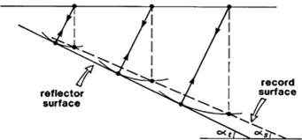
So far we have only considered interfaces which are approximately horizontal. However, the subsurface may consist of dipping layers. This can lead to challenges when attempting to interpret reflections in the data.

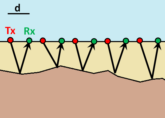
For a zero-offset survey, we can see that the reflected signal returns at an angle. This is because the reflection happens perpendicular to the surface of the interface in this case. As a result, the two-way travel time does not correspond to the depth of the interface. Instead, it corresponds to the minimum travel distance. If we assume the reflected signal gives us the vertical distance to the interface, we will under-estimate the dip of the interface.

Fig. 14 Reflections from a dipping layer for a common-offset survey.

Migration Correction

The true dip of the interface can be recovered using circular arcs. To apply the correction (assuming you have obtained the velocity of the top-layer from the direct ground wave or other means):

1. Obtain the distance from the two-way travel time of the reflection. Assume this represents the vertical distance to the interface. Doing so will give you the dashed line shown in the figure above.

2. For each Tx-Rx position, draw and arc centered at this location, which passes through the under-estimated vertical distance point (found on the dashed line).

3. The true dipping interface is created by drawing a line which intersects all of the arcs at only a single point (black line).

Several of the formulae in this section depend on the propagation velocity \(V\), which varies for different subsurface materials. The following section Propagation Velocities shows a table of propagation velocities for various subsurface materials.

The success of a ground penetrating radar survey, i.e., whether you are able to resolve your target, depends on a number of factors including the type of GPR system that you use as well as the subsurface. In section Expected Resolution of a GPR Survey you will learn how to assess the success of a survey before heading to the field. To understand that section, we will first need to take about the physical parameters at play. This we do in the sections Magnetic Susceptibility, Dielectric Permittivity, and Electrical Conductivity.